Sunday, April 11, 2010
Wednesday, March 10, 2010
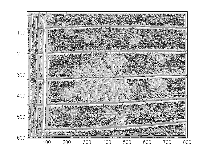
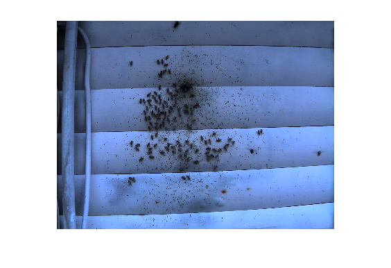
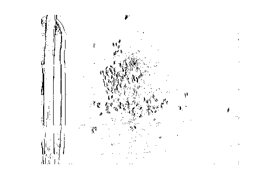
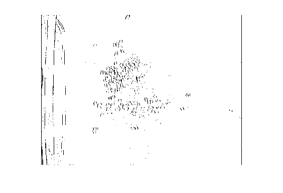
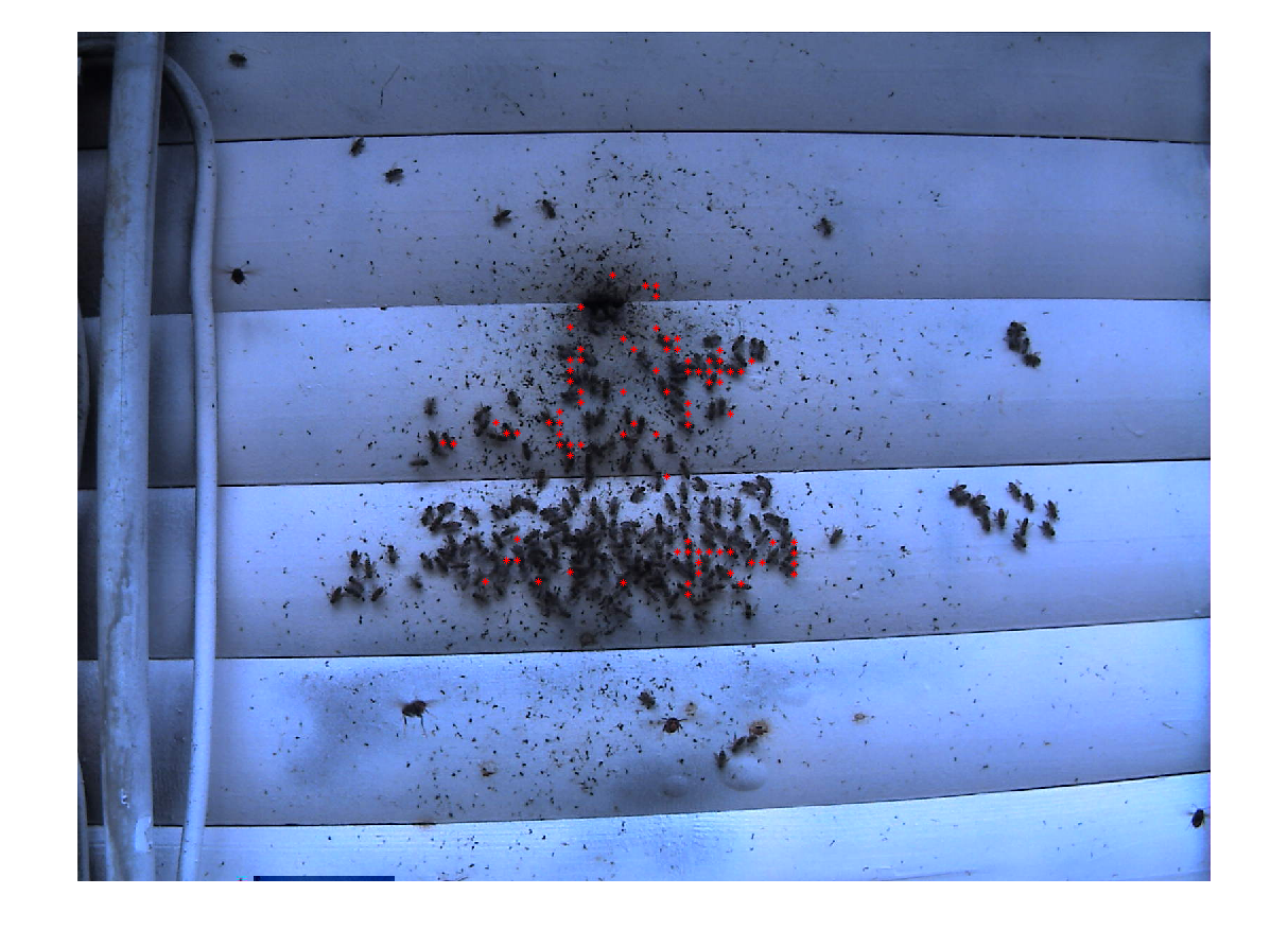
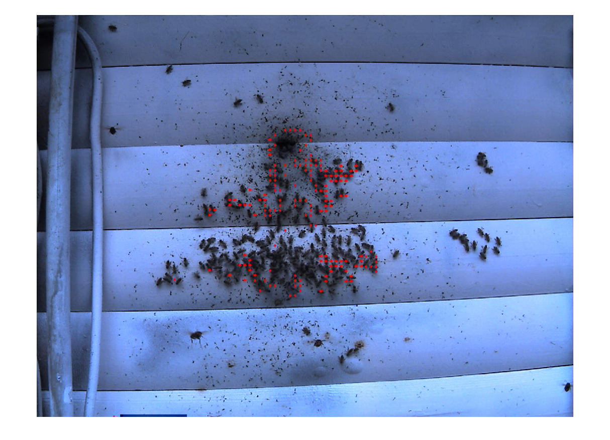
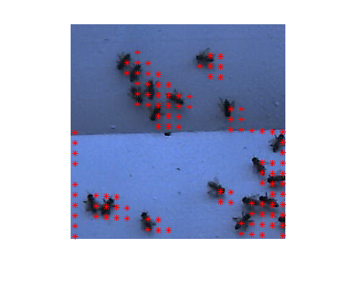
L channel responded index
It looks good on the upper middle region. It was a big block of mud on the original image, but the index table just shows different texture than those bees.
Sunday, March 7, 2010
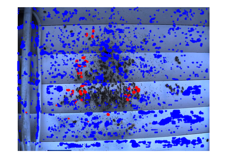
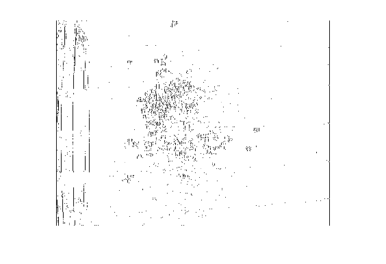
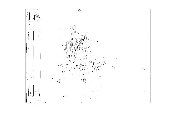
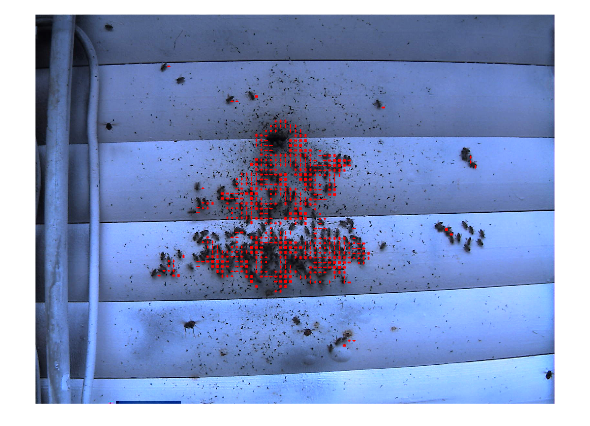
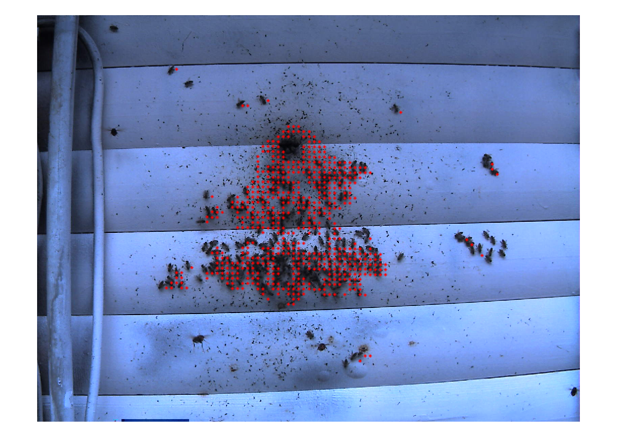
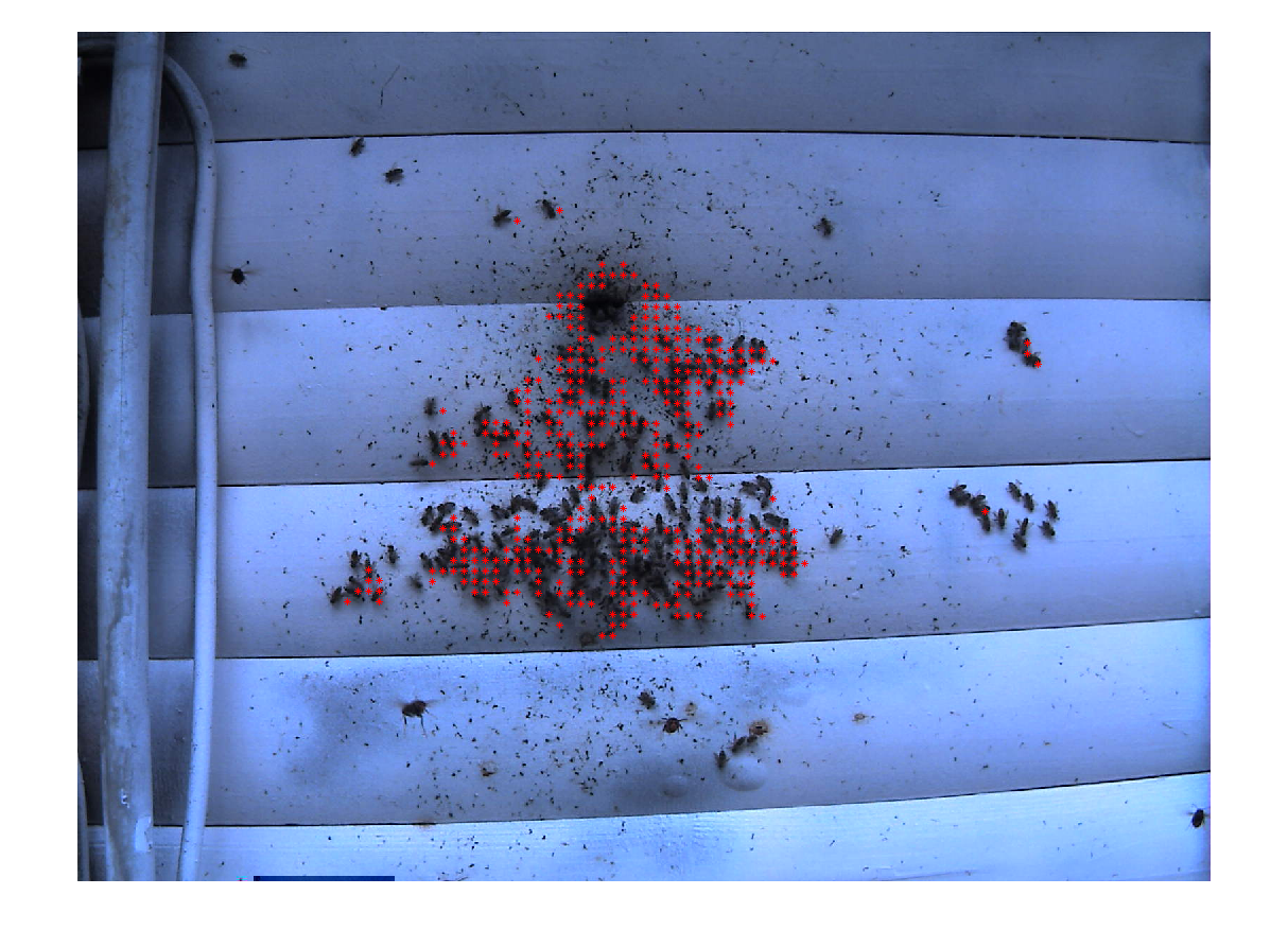
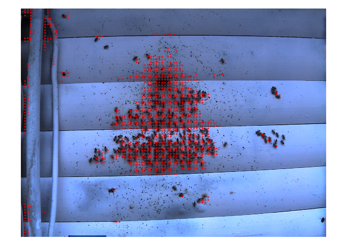
filter bank result
It rejects those negative objects pretty well but also does not fire on the positive bees. Again, I may need a bigger sample size to get an ideal result.
Tuesday, March 2, 2010
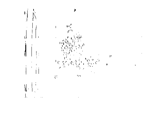
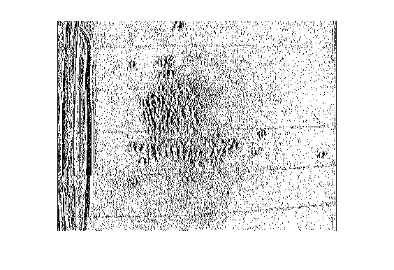
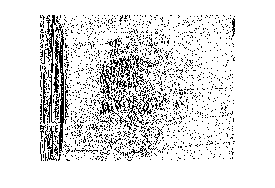
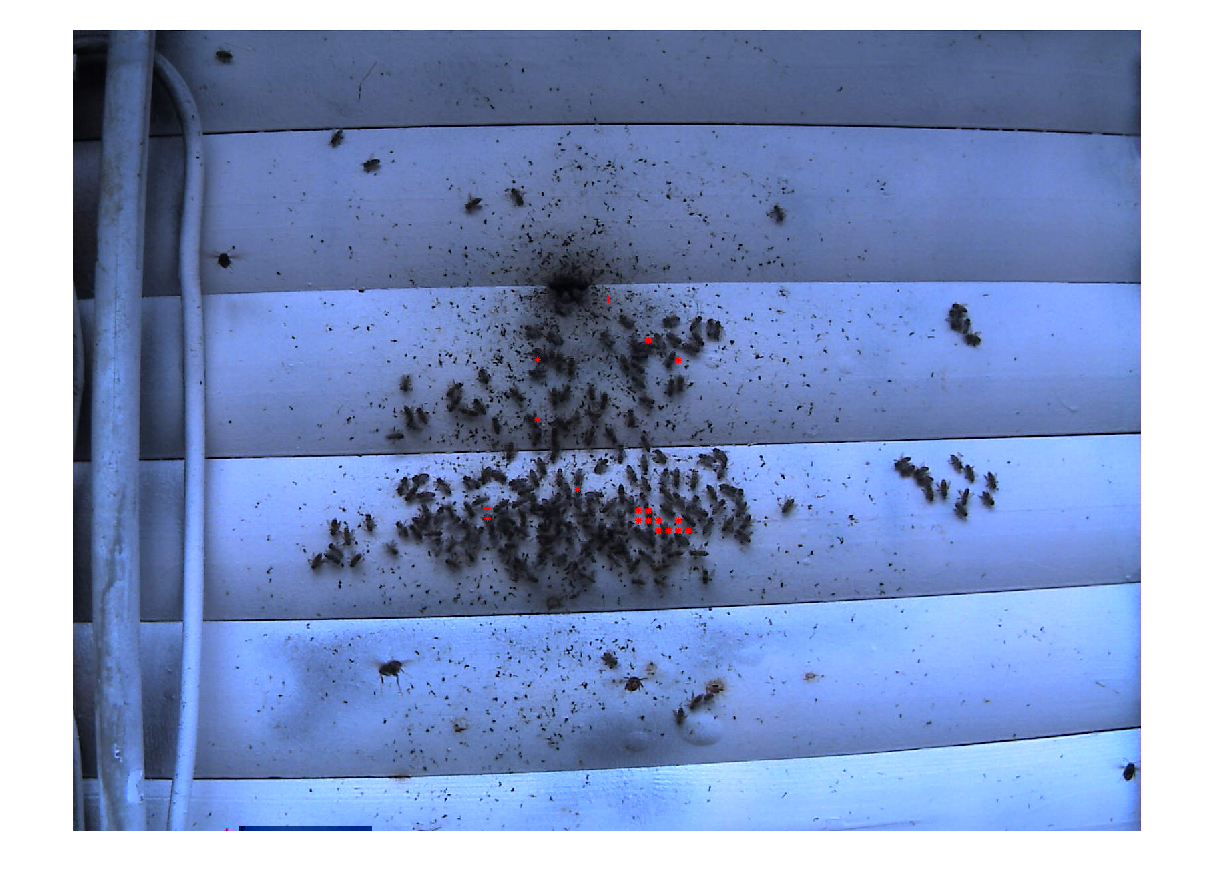
many many clicks
However the red stars at the upper middle of the image is just a big block of mud. I have 3 negative samples to account for that region but it just does not work out.

Monday, March 1, 2010
filter bank

in order to display properly, FB*256 ::should be imagesc() with colormap('gray')::
Apply each of these filters to the image and save the largest *absolute* responded filter's index to an index table. After that do a computer the histogram of these index.
I may have missed something that the result is completely off. At the learning stage I apply the filter to the user selected windows only, while at the finding stage I apply the filters to the entire image. May it be a problem that the convolution of small window is different than convolution of the entire image?
Another problem is that the algorithm is very slow, takes 3 minutes+ to compute.
Wednesday, February 24, 2010

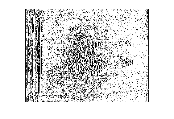

diferent filter results
Only red channel is used. Single channel is filtered by median filter and then convoluted by the different filters. These filters act as edge detectors, and toward the end they are rotated ccw about 45 degrees. These filters are hard coded.
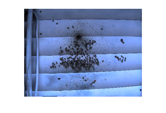
reference image:
filter1
%f = ([1 1 5 7 5 -10 -15 -10 5 7 5 1 1]);
filter2
%f = ([1 1 5 7 5 0 -5 -10 -15 -10 -5 0 5 7 5 1 1]);

filter3
%f = ([ 1 5 7 5 0 -5 -10 -15 -10 -5 0 5 7 5 1]);
filter4
%f = ([ 1 5 7 5 -7 -15 -7 -10 5 7 5 1 ; 1 5 7 5 -10 -7 -15 -7 5 7 5 1]);
filter5
%f = ([ 1 5 7 5 0 -7 -15 -7 -10 0 5 7 5 1 ; 1 5 7 5 0 -10 -7 -15 -7 0 5 7 5 1]);
filter6
%f = ([ 1 5 7 5 0 -7 -15 -7 -3 0 5 7 5 1 ; 1 5 7 5 0 -3 -7 -15 -7 0 5 7 5 1]);
filter7
% f = ([ 1 5 7 5 0 -15 -10 -7 -3 0 5 7 5 1;
% 1 5 7 5 0 -7 -15 -7 -3 0 5 7 5 1 ;
% 1 5 7 5 0 -3 -7 -15 -7 0 5 7 5 1;
% 1 5 7 5 0 -3 -7 -10 -15 0 5 7 5 1]);

filter8
% f = ([ 1 1 5 2 -10 -7 -5 -1 0 1 2 5 1 1;
% 1 5 7 5 0 -15 -10 -7 -3 0 5 7 5 1;
% 1 5 7 5 0 -7 -15 -7 -3 0 5 7 5 1 ;
% 1 5 7 5 0 -3 -7 -15 -7 0 5 7 5 1;
% 1 5 7 5 0 -3 -7 -10 -15 0 5 7 5 1;
% 1 1 5 2 -10 -7 -5 -1 0 1 2 5 1 1]);
filter9
% better:
% f = ([ 1 1 5 2 -10 -7 -5 -1 0 1 2 5 1 1;
% 1 5 7 5 0 -15 -10 -7 -3 0 5 7 5 1;
% 1 5 7 5 0 -7 -15 -7 -3 0 5 7 5 1 ;
% 1 5 7 5 0 -3 -7 -15 -7 0 5 7 5 1;
% 1 5 7 5 0 -3 -7 -10 -15 0 5 7 5 1;
% 1 1 5 2 1 0 -1 -5 -7 -10 2 5 1 1]);
filter10
f = ([ 1 5 2 -7 -5 -2 1 1 1 2 5 2 1 1;
1 1 5 2 -10 -7 -5 -1 0 1 2 5 1 1;
1 5 7 5 0 -15 -10 -7 -3 0 5 7 5 1;
1 5 7 5 0 -7 -15 -7 -3 0 5 7 5 1 ;
1 5 7 5 0 -3 -7 -15 -7 0 5 7 5 1;
1 5 7 5 0 -3 -7 -10 -15 0 5 7 5 1;
1 1 5 2 1 0 -1 -5 -7 -10 2 5 1 1;
1 1 2 5 2 1 1 1 -2 -5 -7 2 5 1]);
Sunday, February 21, 2010
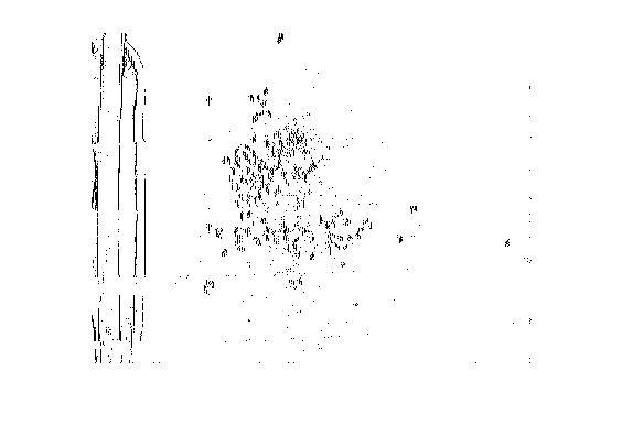
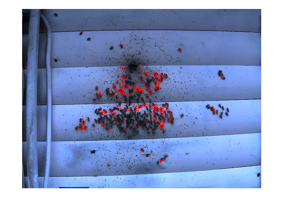
a sample result
The input is filtered before processing the finding stage, and then overlay red start on the original image.
It's obvious that filtering eliminates some false positives, but it also eliminates some overlapping bees.
Again, the learning samples are important for the second stage. I can stack up the learning samples, however, I am not sure whether I should compress them to limit the computation. For now, every learning process starts a new file and abandons all the old data.
Also I think I should head to some kind of texture recognition for the overlapping bees.
Saturday, February 20, 2010
median filtered
Window size 6 pixels overlap 2 pixels.
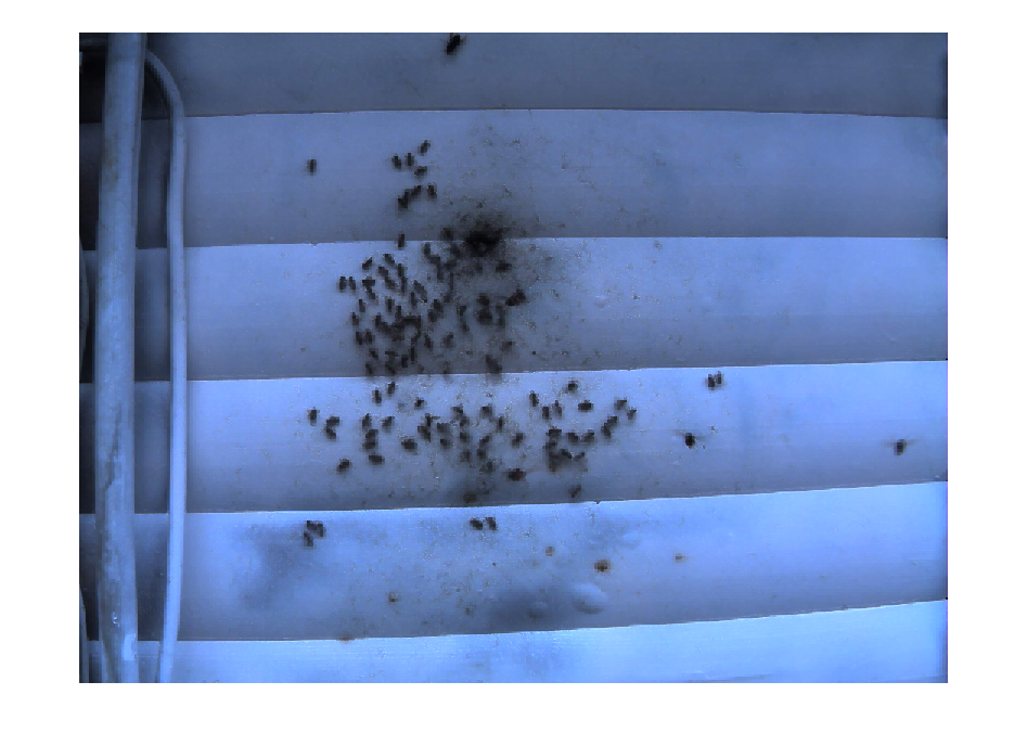 Window size 8 pixels overlap 3 pixels.
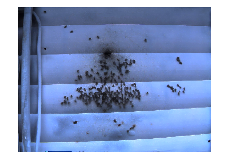
compare to the original image:

Monday, February 15, 2010
Nvidia SIGGRAPH 2009 image processing slide
http://www.slideshare.net/NVIDIA/advances-in-gpu-based-image-processing
Wednesday, February 10, 2010
corr2 is too expensive
positive threshold : negative
0.6 : 1.0
http://farm5.static.flickr.com/4072/4346608685_3b71a707ca_o.png

0.5 : 2.0
http://farm3.static.flickr.com/2790/4346608677_584043b1ed_o.png
0.8 : 2.5
http://farm3.static.flickr.com/2688/4346641775_1578dc4368_o.png

0.8 : 2.0
http://farm3.static.flickr.com/2680/4346641767_f43140b968_o.png

0.8 : 1.5
http://farm3.static.flickr.com/2793/4346641763_2bf8929ac8_o.png
0.8 : 1.0
http://farm3.static.flickr.com/2683/4346641759_81a2639058_o.png
0.7 : 1.0
http://farm5.static.flickr.com/4020/4346641757_152a94b63e_o.png
0.5 : 1.5
http://farm5.static.flickr.com/4047/4346641755_4f6edc29a3_o.png
In sampling phase I intentionally selected bees in a dirty background, for which affected bees in a clean background.
Wednesday, February 3, 2010
problem of multiply bees and a dirty backdrop

This time I pick bees that are in the dirty background and overlay on each other, and try to match them on a similar image. A lot of false positives appear on the respond.
This image cooperates with negative supervise learning.
A window has one score if it has correlation less than 0.5 with the negative samples, greater than 0.9 correlation with the positive samples. Only those with 3 scores are selected.
Wednesday, January 27, 2010
update
user selected samples by learning.m
responds from finding.m
histograms are not comparable when the value of each bin differs. Matlab hist does not provide fixed value range unless user specified. Since I rewrite the histogram function myself and it returns fixed bin size(33) and fixed value range(0:255/33) the histograms are fine.
The blkproc function does not work as I mention in the last post.
This is a useful link for blkproc:
http://www.oit.uci.edu/dcslib/matlab/matlab-v53/help/toolbox/images/blkproc.html
I fix my code to use blkproc(img, [15 15], [8 8], myhist) instead of [30 30] [15 15] windows and border.
An image of 310*310 is used, ceil(310/15) = 21, the windows form a 21*21 grid, and each window overlaps by 8 pixels on its four sides.
to reconstruct the index from a 1D positions,
x = (mod(po(i),21)+1)*15-8; y = (po(i) / 21 + 1)*15-8;
Negative training set is still not enforced in this test. I spend some time to play with the negative result while forgot to load the positive sample back before doing the finding though. r*s spread all over the place.
Tuesday, January 19, 2010
from learning to finding
This is a brief description of the project work flow:
The computer learns interested objects, in our case, bees, from human inputs. The "knowledge" of bee recognition is stored as descriptors in a data structure. On an input image, the computer calculate descriptors in the same fashion as the learning phase, and then finds correlations between the input image and the "knowledge". A highly correlated input indicates that the input is highly possible to be the interested object(bee). As the computer learns more about what can be a bee and what should not be a bee, it can distinguish better and better of the input image.
learning.m is a user interactive script for the program to learn from human: "what is a bee and what isn't". User can double click on the bees (30 for each execution) and the program will store the histogram of color (HOC) and histogram of gradient(HOG) in a [99 30] data structure called positiveResult. Instead of loop over each pixel to accumulate the histogram, his_fast.m uses find function to loop over each bin. Each histogram has only 33 bins vs each image has thousands of pixels. his_fast.m improves its performance significantly by shorten the for-loop. Only A* B* channels and gradient magnitude are used. L channel is ignored and RGB is converted to gray scale before calculation of gradient magnitude. Therefore positiveResult(:, i) is a descriptor of the ith bee.

finding.m detects bees in a given image. The program divide the input image into 30 by 30 small windows and overlap by 15 pixels. For each small window it calculates the HOC and HOG information (his_image [4620 3] for an input image of 273*397), and then compares them with the positiveResult via corr2. his_image(((i-1)*33 + 1):33*i, :) returns a [33 3] descriptor for each window.

Somehow elements in positiveResult have high correlations with unrelated windows. For an instance of "cropped-2-20081212-091900.jpg", posiveResult(:, 1) and flatten version of image(1:33, :) has correlation of 0.86. This is a problem to be resolved.
I threshold to corr2 returns greater than 0.9, and the window is picked only when 3 or more positiveResult agree.
This is a plot for the 75th window compare to 2nd, 3rd, 9th, and 10th positiveResult.

What's next:
A negativeResult can be done in a similar fashion in order to eliminate false positives.
Windows indexing should be built.
Bigger size of positiveResult should be built.
References:
[1] Navneet Dalal and Bill Triggs, Histograms of Oriented Gradients for Human Detection, http://lear.inrialpes.fr/people/triggs/pubs/Dalal-cvpr05.pdf
[2] Stanley Bileschi, Lior Wolf, Image representations beyond histograms of gradients: The role of Gestalt descriptors, http://www.mit.edu/~bileschi/papers/gestalt.pdf
Tuesday, January 5, 2010


Monday, January 4, 2010
Proposal
Abstract
1. Introduction
This project is going to join the on going research of a ecological image database system in California Institute for Telecommunications and Information Technology(Calit2) and Taiwan Forestry Research Institution(TFRI). This project is going to use a computer vision approach to count the number of bees in the image database which were taken from the Shanping Workstation in Taiwan. Furthermore, this project is attempt to make the program as portable as possible so that a on-field camera is able to determine whether or not sending more image or video to the workstation.
2. Milestones
2.1. Week 1
Installation necessary tools (find a possible way of connecting the interfaces such as Java and Matlab) compare the test result of different libaries.
2.2. Week 2
Build a minimum algorithm for bee recognition. Build a practice set of images, identify possible problems for the image set.
2.3. Week 3-4
Build a basic program to distinguish background and the bees. The program should be able to handle different ligtings aross different time of a day as well.
2.4. Week 5
Add wasp recognition to the prorgam in order to triger the wasp attack event.
2.5. Week 6-8
Add aglinment across different images, so that the change of camera viewpoint. The program should be able to handle external events (such as birds or other objects in the scene) and fatal errors (completely dark image or camera outrage)
2.6. Week 8-10
Testing and integration phrase. It is expected to run this program on an embeded computer with MIPS processor. CPU and memory usage should be optimized.
3. Problems to be solved
3.1. How to distinguish background and the objects of interest
By observing the images, the good side is backgrounds do not change frequently, but the down side is backgrounds containt a lot of distractions (black dots which look very much alike to a bee)
3.2. How to handle the cases when bees group together and stack on top of each other
As illustrated in Figure 1. when bees are closed to each other.
When a wasp attacks the bees, bees group together around the wasp and vibrate in order to defence their nest. If a wasp can be recognize the program should be able to triger the camera and perform a video capture [3].
3.3. Camera alignment and lighting problems.
It would be much easier to perform the counting task if the program is able to take the background away. However, camera position changes over time because of wind, gravity or any other external force. For anther thing, lighting of the scene changes over time. In order to ignore the background, a baseline should be drawn.
3.4. On field camera integration problems
The final report will adress difficulties and problems of integration with a realtime on field camera.
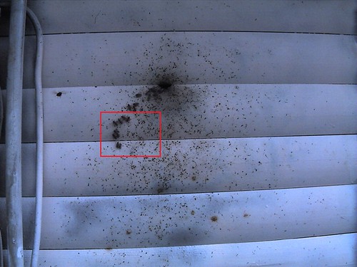

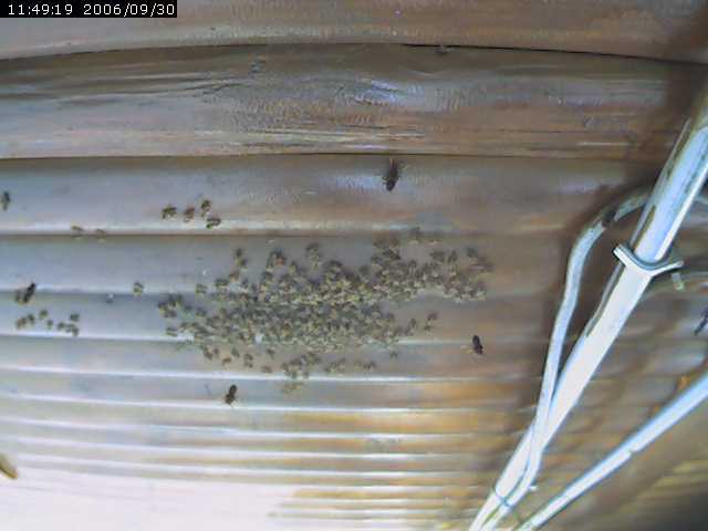
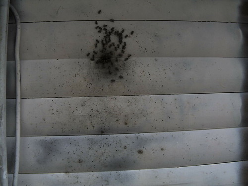
Figure1: Sample image from TFRI
Upper: A sample image from TFRI website taken at Feb 04, 2009 7:02 AM [1] original size 1600*1200 pixels
Lower: Cropped image from the upper image
4. Softwares to build upon
This project is going to be developed in Matlab and Java, and interfaced with the open source middle ware Data Turbine[2], specifically, Ring Buffered Network Bus (RBNB) and/or Realtime Data Viewer (RDV) [4].
5. Datasets
This project will use the images from archiving gallery of Shanping workstation of TFRI [1]. Image resolution is 1600*1200 since September 2008. White painted background since December 2008.
References
[1] Sensor Archiving Gallery of Shanping Workstation http://srb2.tfri.gov.tw/wsn/
[2] Open Source DataTurbine Initiative: Streaming Data Middleware and Applications, Tony Fountain, Sameer Tilak, Jane Rutherford and delegation from Canada, (2008)
[3] Ecological image databases: From the webcam to the researcher, John Porter, Chau-Chin Lin, David E. Smith, Sheng-Shan Lu (2009)
[4] A visualization environment for scientific and engineering data http://code.google.com/p/rdv/